Pizza2vec

Topic Modeling in Yelp

One of my favorite things in this wonderful world is a good pizza. Arguably my first real love, pizza has taught me some of the most important things to be learned in life. Beyond making dinner suggestions incredibly easy, good pizza will ALWAYS make that list. Also, I was fortunate enough to gain some foundational business experience as a teen in cozy St. Cloud, MN, where I managed a local pizza shop.

I have only been to New York City once in my life, for a weekend, and pizza became a focal point of the trip. Knowing where to go was really easy thanks to some solid suggestions from my graduate school percussion teacher who tipped me off to such greats as Lombardi’s, the oldest pizzaria in NYC, and Angelos. In addition to spending time with friends, the awesome food made the trip that much more memorable and fun.

I love checking out great local pizza spots when I travel, but I am usually way too busy to find the most relevant reviews for what I want at a given time and place. So I wondered, could I create a clustered topic model for pizza reviews on Yelp?

It turns out Yelp offers a slice of their data for academic purposes as well as an API. To test the pizza waters in Yelp land, I am going to use their academic dataset first to see if I can prototype something useful before considering a more robust solution.

Read the data into Python

The data that was used for the post can be downloaded from the following URL Yelp Dataset. The data is available in both SQL and JSON, I chose to download the JSON version. I read the data into python with JSON package I used codecs to iterate through the JSON files and write the data to disk. Instead of topic modeling on the entire roughly 3 million review restaurants, I chose instead to subset to reviews that contained the word pizza. There is a phenomenal pycon presentation from Patrick Harrison on modern natural language available here. I used the same general approach as his tutorial and additionally added clustering to the word vectors to make the results more interpretable. I highly recommend watching that video if you are interested in learning more about modern natural language processing. A general snippet for reading the business and review data files is shown below. The code used to read, clean, and model the data can be found in my github repo using this link.

import os
import codecs

dir = os.path.join('..', 'data')

filepath = os.path.join(dir,'business.json')

with codecs.open(filepath, encoding='utf_8') as f:
    f.readline() 

Preparing the text for modeling

Text data can be very highly dimensional. If proper steps are not taken to clean the text data, then one should not expect to have a very accurate or useful model. To clean the data I tokenized the spaces and punctuations and lemmatized the data. Lemmatization being is the process of text normalization for casing of letters contractions and whatnot. I also created uni, bi, and trigram sentences, this combines common words found in the corpus together to a single word representation of the word such as ny_style_pizza. All of the natural language processing has thus far been achieved using the python package Spacy. I could have built my own stopword vocabulary in Spacy, but that would require building my own stopword dictionary. So I chose NLTK to remove stopwords, as they have a list ready to use out of the box. Finally I used Latent Direlecht Allocation to transform the data into a bag-of-words representation.

Word2vec

The first step in modeling the data was to use the package Gensim to represent the words in a highly dimensional vector space to create a continuous bag-of-words word2vec model. This uses a discriminate approach using a binary-logistic regression-classification object for target words. ${\mathbf{w}}_{\mathbf{t}}$, and $\mathbf{k}$ imaginary words $\stackrel{~<!--\; ~\; -->}{\mathbf{w}}$

Below is an illustration of what is happening in continuous bag-of-words modeling.

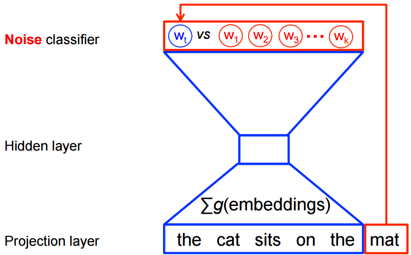
This maximization objective is represented mathematically below

where ${\mathbf{Q}}_{\mathbf{\theta <!--\; \theta \; -->}}\mathbf{(}\mathbf{D}\mathbf{=}\mathbf{1}\mathbf{|}\mathbf{w}\mathbf{,}\mathbf{h}\mathbf{)}$ is binary logistic regression probabilty of seeing $\mathbf{w}$ in context $\mathbf{h}$ of dataset $\mathbf{D}$ in embedded learned vectors $\mathbf{\theta <!--\; \theta \; -->}$ where $\mathbf{k}$ represents noise words.

The images and mathML code were borrowed from Tensorflow. Tensorflow has awesome documentation; go there and or their github repositories to learn more.

t-sne

Next we use a dimension reduction technique called t-distributed neighbor embedding, t-sne. This reduces the dimensional space to an x-y coordinate space, and similar topic words will be clustered together. Unlike PCA dimension reduction, t-sne is based on probability distributions with random walk on neighborhood graphs to retain both the local and global structrues in the data. The first step is to convert the high-dimensional Euclidean distances between points into conditional probabilities showing similarities see the mathematical representation below:

For high dimensionality space, the similarity of 2 points are decided in proportion to their probabilty density centered under a Gaussian at xi. and .

For low dimensionality, the conditional probabilty is mathematically represented below:

Finally we will look at Perplexity, which is defined mathematically below as 2 raised to the Shannon entropy value below:

Perplexity can be thought of as a high dimensionality smoothing mechanisim. The images above were borrowed from the t-sne wikipedia pages and this blog

Clustering

It is very common to use KMeans as a clustering solution after performing t-sne reduction. I experimented first computing a variety of kernels and found, based on the silhouette scores, that 3 and 7 kernels did the best. Both of those solutions mis-clustered some obvious kernels though, splitting them in half. Next I tried DBSCAN but that solution had trouble discerning a signal from the noise creating 125 different kernels where the vast majority of observations were assigned to one cluster and only a few words were assigned to the remaining 124 kernels.

Spectral Clustering, a clear winner! The code below represents how I trained the clustering algorithm using the python package sklearn.

# Creating a Spectral Clustering model

from sklearn.cluster import SpectralClustering
sc = SpectralClustering(affinity = 'nearest_neighbors', assign_labels = 'kmeans'

Going a bit deeper, spectral clustering varies from kmeans in how the distances are computed. Geometrically speaking, Kmeans uses the distance between points where as Spectral Clustering uses the graph distance, in this case nearest-neighbor. In addition I specified kmeans label as opposed to discrete, which allows for finer granularity of clustering. It can prove to be unstable and unreproducible, but seems to work remarkably well for this problem.

Visualization

The interactive plot below was created in Bokeh. In order to get the plot to have all the functionality I wanted, the size of the html code ended up being really huge. To optimze the performance, I used WebGL back which can be enabled in one line of code.

Great, so I have an interactive plot that looks like a cheap knock off of a google chrome logo; so what can I do with this?

If we examine the clusters closely we can see that the combination of t-sne/spectral clustering came up with some really interesting results! Below are my interpretations of what each of the clusters represent.

The words represented in the follow topic clusters:

• Black Cluster. There is a bit of pareidolia for me with this cluster. The right eye of this perhaps inebriated smiley face is devoted to booze and the left eye is a cluster related to deserts. The mouth or lower region is related to mouth feel, texture, and presentation.

• Yellow Cluster. Words in this cluster are related to price. This is a pretty isolated cluster, relatively speaking, and is very dense compared to the spread of the other clusters.

• Navy Cluster. When I started this project I was pretty sure that in some shape or form I would be able to identify the cliche snoody review, well this cluster seems to be the key. Generally speaking this cluster appears to be related to service, where the many of the topic words in this space seem non-satisfactory reviews. It makes sense that people would be a bit more affected by the service then the actual food at a restaurant. Having been on both sides of this eqution I know there can be very unreasonable customers and also unacceptable service from some who clearly does not care you or your food. I wasn’t totally sure if these types of topic words would be more general or within a more specific cluster such as this one or the food cluster in red.

• Pink Cluster. Pink clustered words are related to hours and events. There is a dense section in this area designated to sporting events. My gut would have been to guess that sporting events would some how be related to drinks and bars, but being associated with events and timing actually makes much more sense. There are also 2 distinct dense subclusters around time in minutes, likely relating to delivery time, seating time, or the time it took to prepare a meal in general. The other is related to time of day, this would likely related to specials like happy hour and events like bands and what not.

• Orange Cluster. The words in this cluster are related to a place or location. Most of the words have to do with street names and cities.

• Blue Cluster. This cluster is predominately related to foriegn words, with 2 dense clusters for French and German.

• Red Cluster. This cluster is related to ingredients and food items. There is a fairly dense and wide area that sees to be mainly bar and american grill and fryer style food items which has a tail from sushi style items to asian foods. Authentic Italian has its own fairly isolated dense cluster within this red cluster. Other styles of items seem to be outliers in this representation of the data.

• Green Cluster. The words in this cluster have less affinity than those in the other groups. These appear to be mostly words that are a bit more general than some of the other clusters. The densest looking cluster, in the lower right region, is all related to names. The next densest layer was table types, mostly fine dining tables and the next was for the floor of the building, most likely for the location of the restaurant.

Conclusion

This model could be used for a number of applications. If this were a project for a real company/problem, this approach could be used to pipe customers to various treatments based on their reviewing behavior. An additional step would be needed for that. Say someone posts about upscale entrees, grouped in red in the plot above, then your engagement with those customers may be more focused on menu items, where ash customers who reviews are more oriented towards price you may want to send more coupons or something. A common approach would be to create word2vecs for each review and average them, then preform t-sne. A hybird approach could be used as well, where the most import word topics are calculated for all of the reviews together, then calculate an averaged word2vec for each review and compare to the overall most important word topics.

Even though tuning this model took some time for me to optimize and to try out different algorithms, it is still amazing to me that the models themselves can find such robust patterns in the data. While this was trained on the academic data set, I am seriously considering creating a version of this model with their API. I absolutely love the idea of tailoring my Yelp search to topics that I am interested in at any given time. Say I am in Portland and want to get a local brew with my pie, I could apply that model to only search for beer related pizza review! Perhaps I am in chicago and want the most upscale pizza I can find, I could use that cluster to find reviews in Chicago that are relevant.